Learning Using Thinned Networks: A Crowdsourcing Phenomena in Reservoir Computing

My name is Joseph Wilkes and I’ll be presenting on exploring the ability of Reservoir computers to learn chaotic systems

I would like to thank my team Dr. Benjamin Webb and DJ Passey and Joseph Jamieson. Feel free to email us.

I would also like to thank the National Science Foundation for sponsoring me to be a part of this conference.

As an overview first I want to talk about the Lorenz attractor, then the reservoir computer model. Then I want to introduce our main hypothesis as it relates to thinning the internal network of the reservoir computer, then I want to describe a significant discovery. The spectral radius and sparsity of a network interact to impact predictability. Then we’ll talk about future research avenues, and then we’ll have time to answer questions.

We are attempting to predict the unpredictable. But what exactly are we trying to predict?

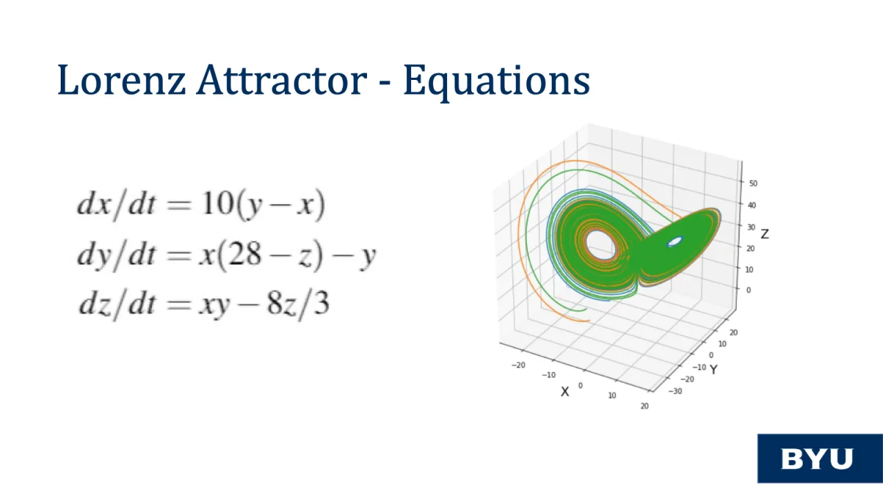
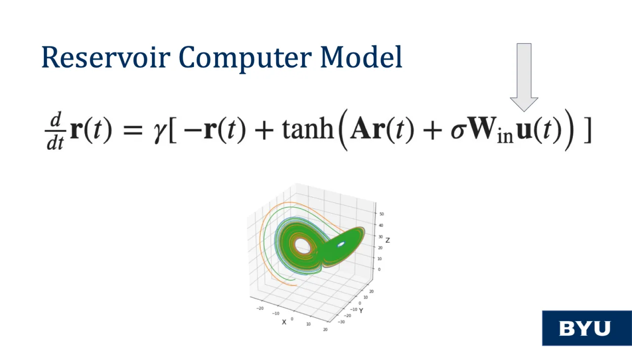
We are trying to predict on the Lorenz attractor. The Lorenz attractor is a canonical example of a chaotic system in which the behavior is extremely dependent upon initial conditions. Thus two particles with incredibly similar initial conditions will inevitably have diverging trajectories. There are many captivating videos of this behavior online which I recommend that you look up. We are trying to predict the trajectory of a particle on this attractor. The Wikipedia webpage on the Lorenz system states: “In the absence of perfect knowledge of the initial conditions, our ability to predict its future course will always fail. This underscores [the fact] that physical systems can be completely deterministic and yet still be inherently unpredictable even in the absence of quantum effects.” Thus we are trying to predict the unpredictable. This chaotic behavior is governed by a system of ordinary differential equations as depicted on the left as is illustrated on the right.

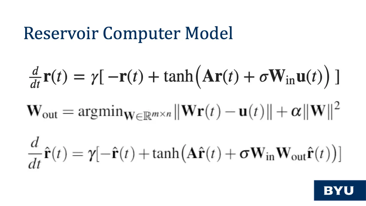
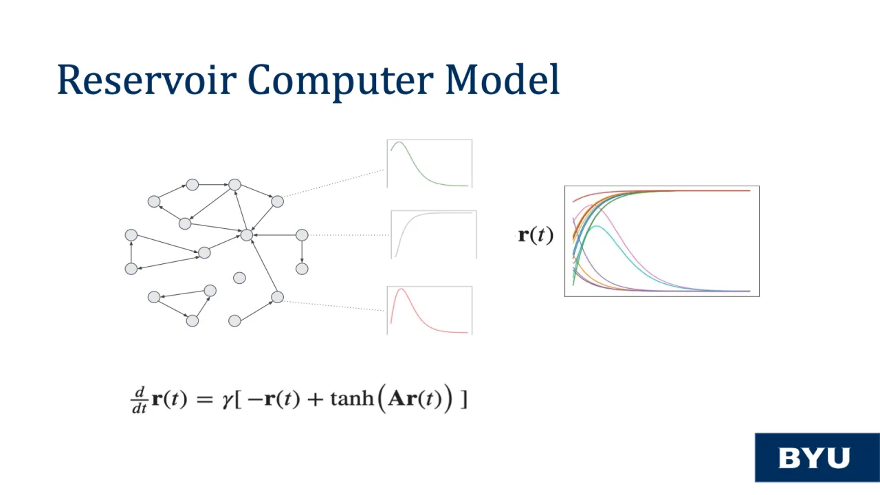
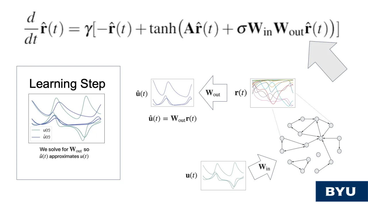
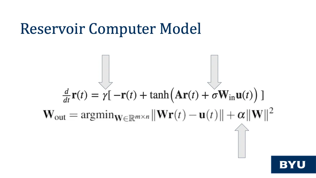
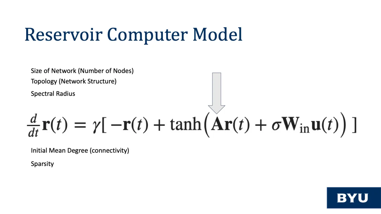
Now I’d like to describe the machine learning model, called the reservoir computer, that we use for prediction in this chaotic system. There are three governing equations in this model. Although overwhelming initially when you first see these equations, we will dissect the essential parts to illustrate what is going on under the hood.

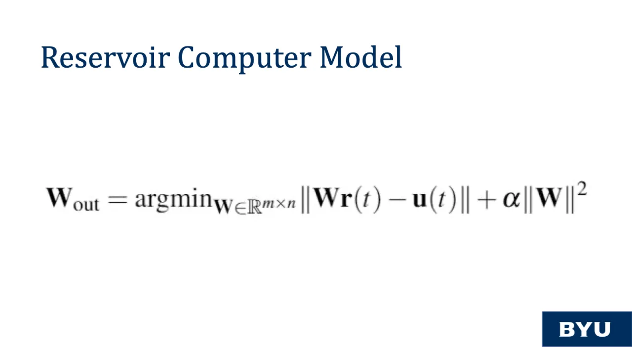
The first equation, primarily, is a differential equation that describes the framework of the reservoir computer. Second is a minimization equation used for learning the optimal matrix that will allow the dynamics of the reservoir computer to be translated back to the Lorenz System. Lastly is the combination of the first two equations in order to make predictions. We will investigate these equations more in depth now.

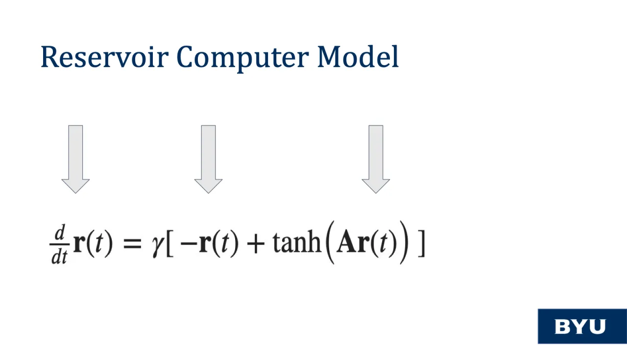
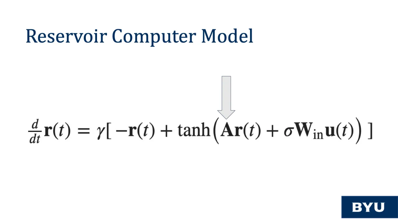
The reservoir computer, in its simplest form, merely describes the dynamic node states and their values as a function of time. This is before receiving any input or information regarding the Lorenz Attractor.

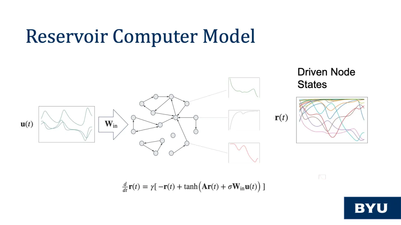
We add in the vector u(t) to drive the reservoir computer by the 3 dimensional trajectory of a particle in orbit on the Lorenz attractor.

The W_in matrix is a fixed linear mapping that maps the training signal from the Lorenz coordinates into the n-node states.

This second equation describes the learning phase of the machine learning process. We calculated the matrix that minimizes the difference between the mapping of our node states and the training signal. You will probably notice the regularization term which penalizes the optimal W_out matrix from becoming ill-conditioned or overfitting given the training signal.

Once we have the W_out matrix we are able to map the dynamics of the reservoir computer back to the Lorenz system in order to predict the trajectory of the particle. Next, as seen here, we then replace the training signal u(t) with this mapping by W_out of the node states to propagate the node states as time advances.

Now to introduce our own revolutionary adjustment of the model! Before describing our main hypothesis I want to review another relevant component of the reservoir computer equation.

In this equation, there are several hyper-parameters: Gamma, Sigma, and Alpha, of which we could talk at great length about the impact of these hyper-parameters, but...

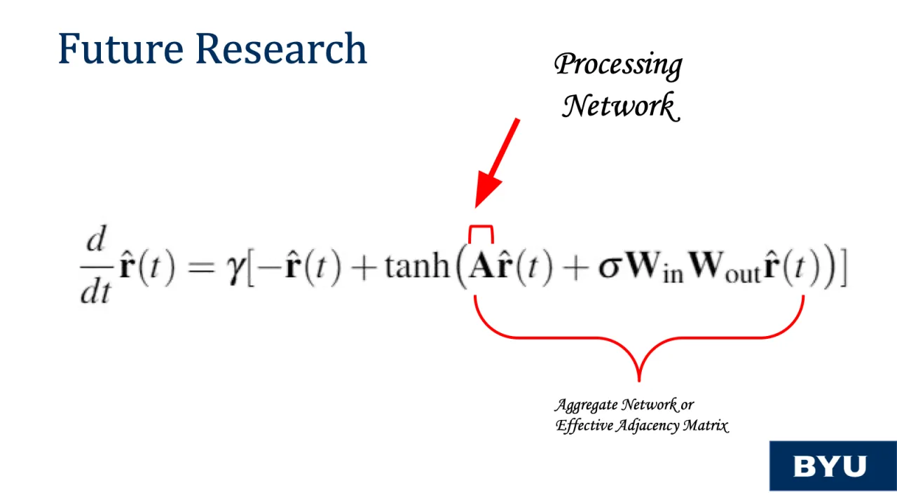
The aspect of the equation that I especially want to bring to your attention is the A matrix.

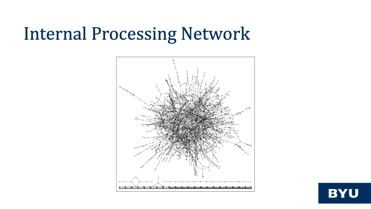
This is the internal network that describes the structure of the nodes. We call this the processing network.

There are 5 other hyper-parameters associated with the processing network. The size of the network, the topology or network structure, the spectral radius, the initial mean degree or connectivity of the matrix, and then a parameter we will discuss more which is the sparsity of the matrix.

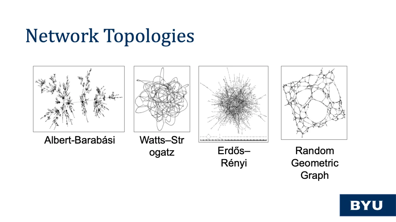
There are network topologies that are found in the real-world today like Albert–Barabási, Watts–Strogatz, Erdős–Rényi, and Random Geometric to name a few. We won’t discuss the primary characteristics of each of these topologies for lack of time but in our research we do consider each of these topologies (and more) and their characteristics in depth.

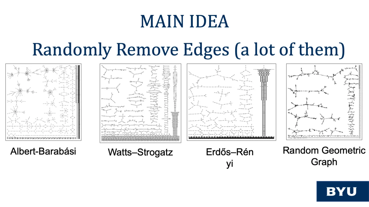
One network characteristic that many consider to be of note is network connectivity. We can see their point, and we still had the audacity to explore the resiliency of the reservoir computer as edges are randomly removed from the internal adjacency matrix. We fractured and obliterated these networks.

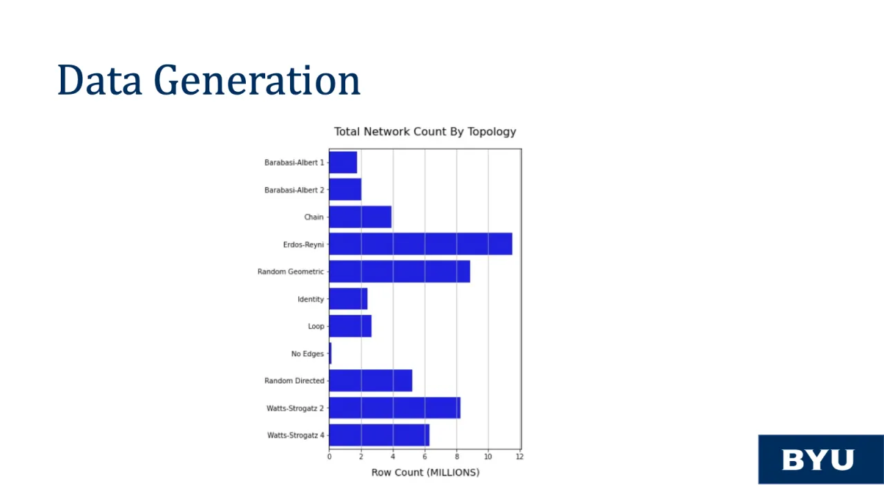
To thoroughly test and experiment in this regard we produced tens of millions of simulations of the reservoir computer with ranges of hyper-parameter values.

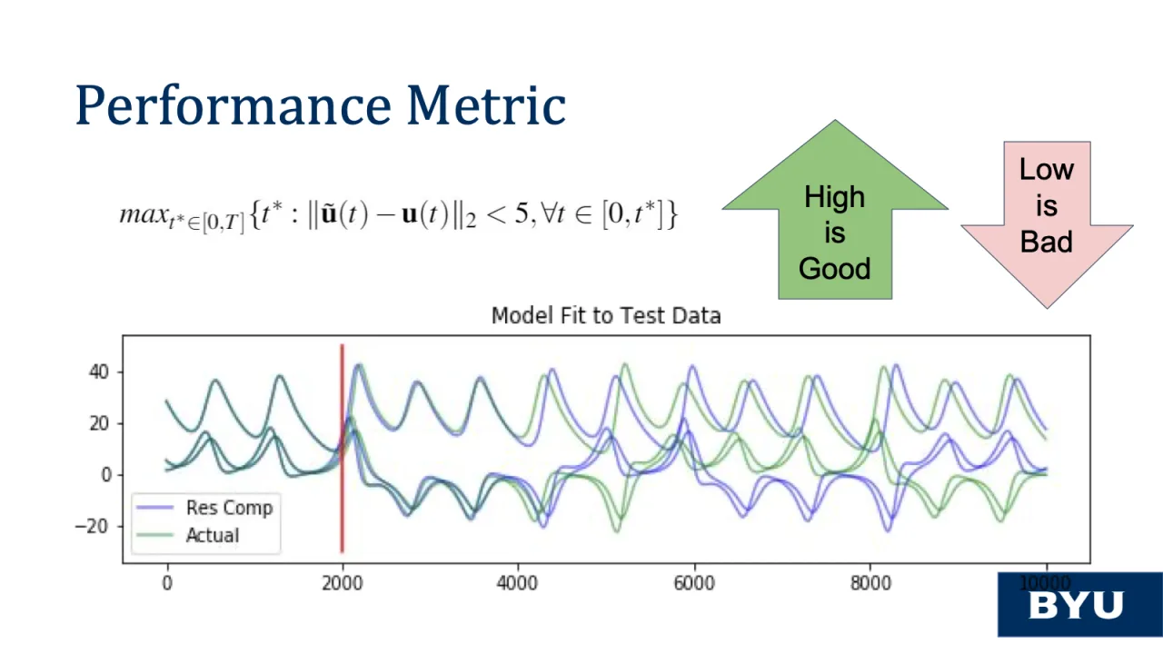
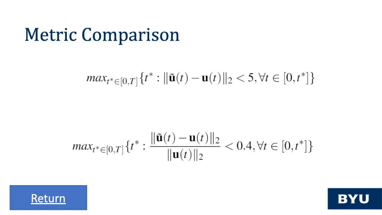
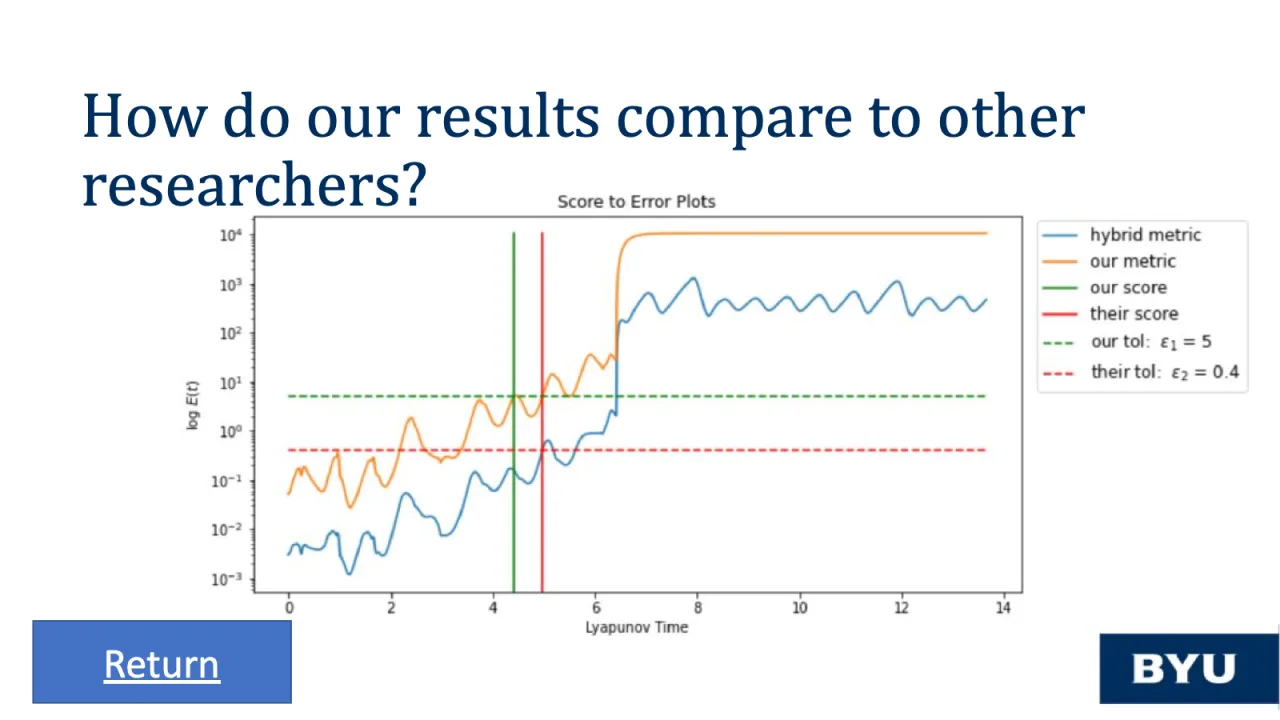
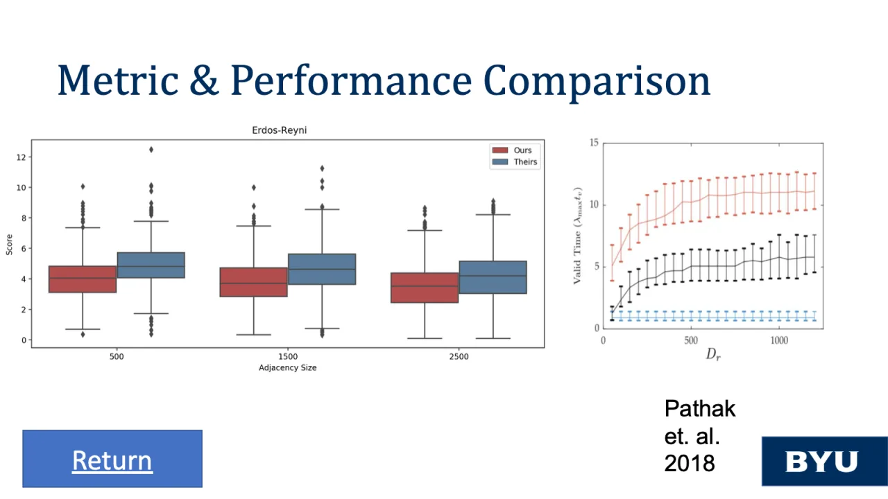
But in these experiments, how should we measure the effectiveness of an individual simulation compared to another? The metric we used, and note there are many other metrics that could have been used, the metric that we used, is what we call the accuracy duration or Valid Prediction Time (VPT). This metric describes the length of time, where the prediction is within a tolerance of the true solution. Simply stated, a high VPT is good, and a low VPT is bad.

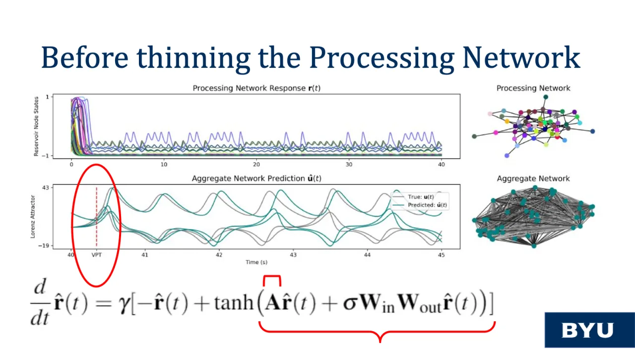
Over the next two slides we will compare an individual simulation. We can see in the top left - the node states during training prior to solving for (or learning) the W_out Matrix, on the top right we see the processing network or the A matrix as listed in the equation - prior to thinning. On the bottom right is the aggregated network or effective adjacency matrix which is the processing network plus the scaled version of the mapping of the input signal. On the bottom left is the comparison of the predicted versus the true trajectory for each dimension of the 3 dimensional signal which illustrates its Valid Prediction Time - our primary scoring metric.

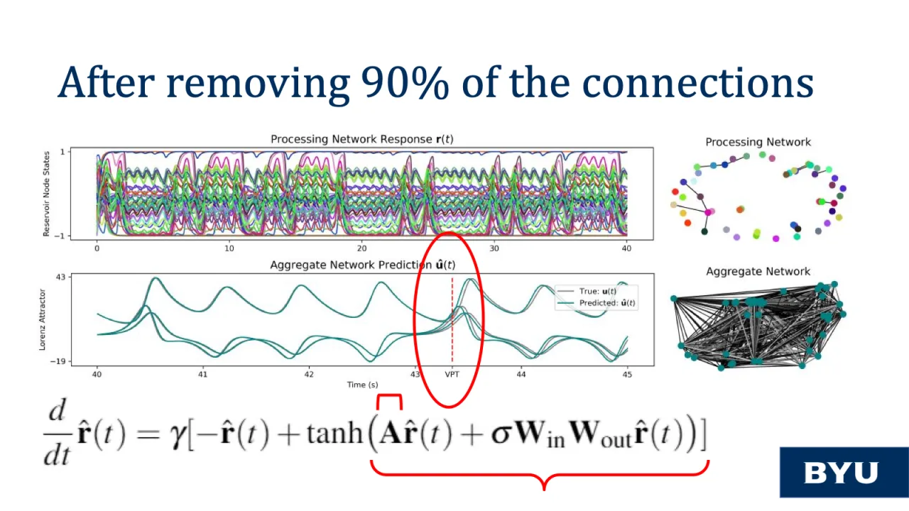
Next we will look at a version of this simulation where the processing network has had 90% of its edges removed. You will notice a few things. On the top left the node states seem to be more active than before, on the top right you’ll see the thinned processing & aggregated networks. And then you’ll see the comparison of trajectories with the resultant Valid Prediction Time. There is an astounding increase in VPT. The x-axis starts at 40 seconds. That’s the point in time when training ended. The range of the x-axis from 40 to 45 seconds is when we’ve introduced the W_out matrix and the reservoir computer is driving itself. Thus for the VPT to go from 40.34 seconds to 43.34 seconds (which we can disregard the 40 seconds of training), this 3 second difference represents an increase of 10 times the accuracy duration just by introducing more sparsity into the network. I know that’s a lot of information to digest in a short amount of time but I hope I can communicate that these results are remarkable.

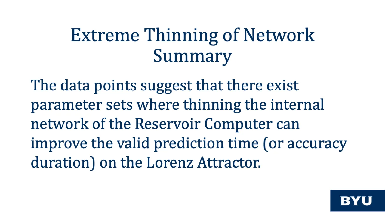
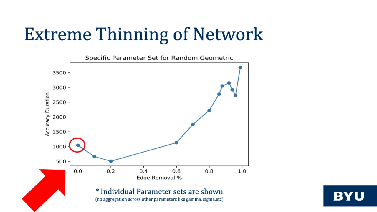
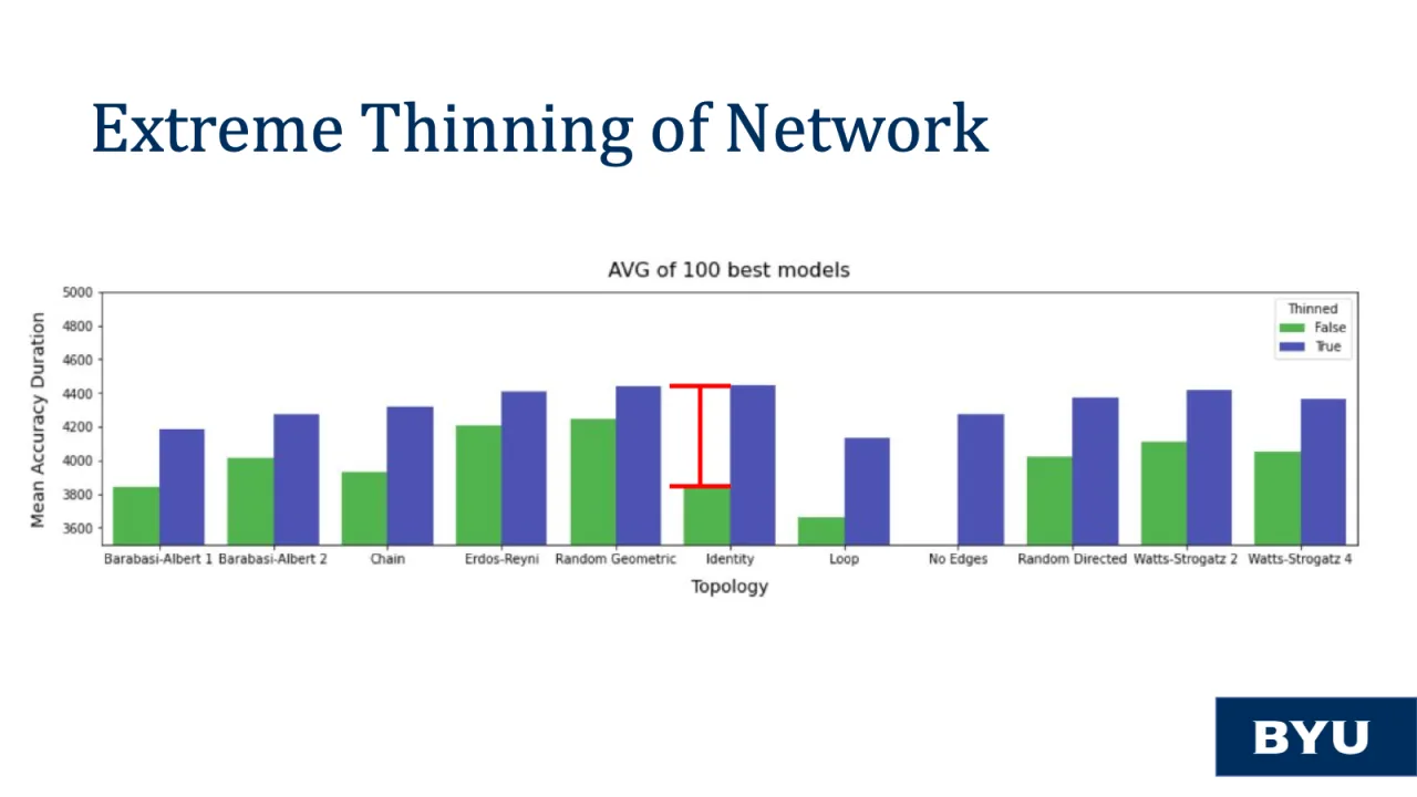
The data points suggest that there exist parameter sets where thinning the internal network of the Reservoir Computer can improve the valid prediction time (or accuracy duration) on the Lorenz Attractor.

We are exploring an analogy that relates this idea of thinning to crowdsourcing. The idea that many amateurs can be greater than one professional or expert. This idea is discussed more in depth in our research paper. This may also suggest a contrast between information processing & information learning or generalization. Although a highly connected network may be able to process large amounts of information like the world wide web there may be more to learning than just connectivity. We are about to see yet another level of this discovery that can lead to improved model design principles as we investigate the relationship between spectral radius and network sparsity.

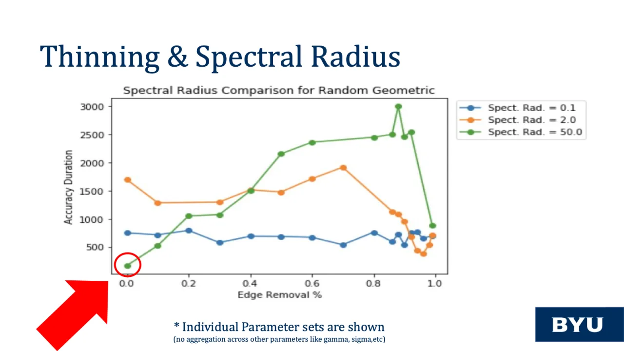
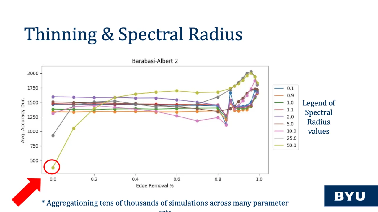
In the following 2 visuals, the Valid Prediction Time or Accuracy duration has been discretized from seconds to thousandths of a second as shown on the Y-axis. And the Edge Removal % is shown on the x-axis. Note that the spectral radius for the simulations is shown in the legend on the right.

A lot of current literature suggests that spectral radius should be near one. This seems intuitive in that reservoir computers with a high spectral radius perform poorly on Chaotic systems when the internal networks are dense & very connected as seen by the most bottom left point; However, We see an underdog phenomenon where the higher spectral radius model goes from being the worst predictor to being the best predictor as the network is thinned.

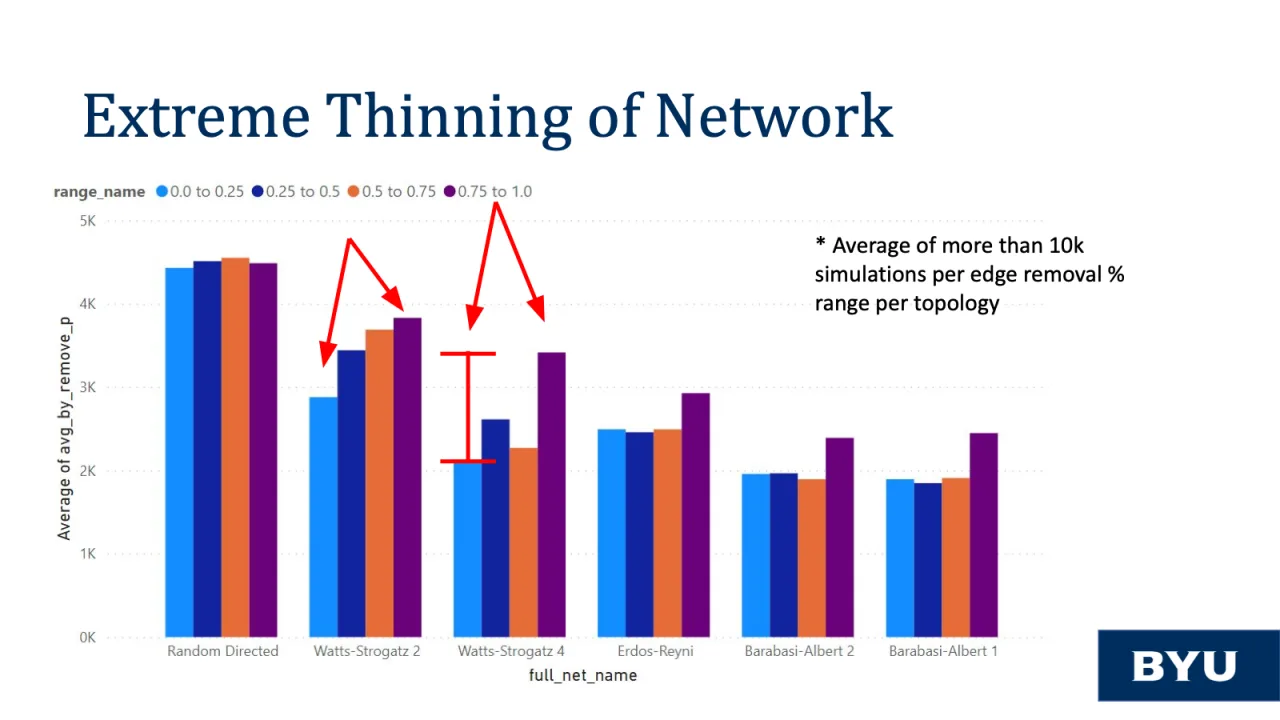
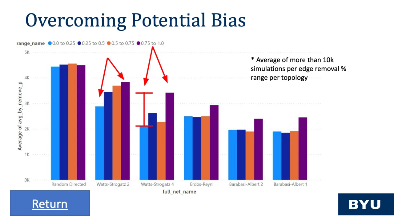
This is a rather revolutionary idea that holds true as we aggregate tens of thousands of simulations for each edge removal percentage value. This trend was present in many different topologies.

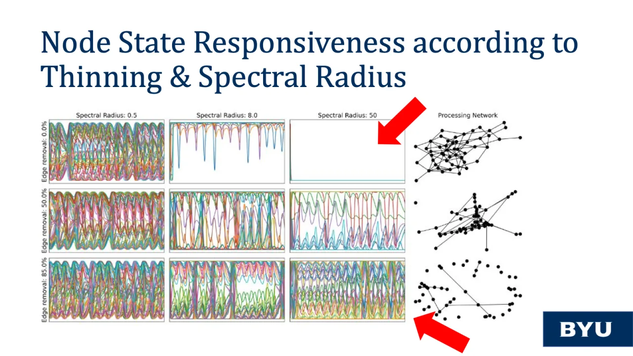
Why don’t we investigate the node states of the reservoir computer as we increase both spectral radius for a dense & vastly connected network? we can see that according to the top right subplot that the node states are very unresponsive to the input signal whereas in the bottom right subplot as the edge removal % is increased and the spectral radius is 50, then we see that the node states are remarkably responsive to the input signal.

The data points suggest that Reservoir computers with dense internal networks and high spectral radius can be really bad predictors whereas extremely sparse networks with high spectral radius can be the best of predictors.

For future research, we can take these discoveries of thinning out the A-Matrix, or the processing network, and we can explore them further by intentionally thinning out the effective adjacency matrix, or the aggregate network even more. Initial investigations suggest that this too can lead to improvements in Valid Prediction Time on Chaotic Systems.